How Can Motion Have a Speed at One Instant?

A dashboard can display 47 miles per hour at 3:14:08 PM. That reading creates a small mathematical problem. During one instant, no time passes. The car travels no distance. The familiar calculation

$$\text{speed}=\frac{\text{distance traveled}}{\text{elapsed time}}$$

appears to become $0/0$, which is undefined.

Physical speed sensors sample motion over short intervals. Mathematics asks what those measurements would approach if the intervals could shrink without end. The resulting local rate of change is called a derivative.

Begin with a speed we can calculate

Suppose an object moves along a straight track. Its position after $t$ seconds is

$$s(t)=t^2 \text{ meters}.$$

At $t=1$, the object is at $s(1)=1$ meter. One second later, at $t=2$, it is at $s(2)=4$ meters. Its average velocity over that interval is

$$\frac{s(2)-s(1)}{2-1} =\frac{4-1}{1} =3 \text{ meters per second}.$$

That calculation measures a whole second. To examine motion nearer to $t=1$, choose a nonzero time offset named $h$. The second time is $1+h$, and the average velocity becomes

$$\frac{s(1+h)-s(1)}{h}.$$

For $s(t)=t^2$, several choices of $h$ give:

$h$ in seconds	Interval	Average velocity
$1$	from $1$ to $2$	$3$ m/s
$0.5$	from $1$ to $1.5$	$2.5$ m/s
$0.1$	from $1$ to $1.1$	$2.1$ m/s
$-0.1$	from $0.9$ to $1$	$1.9$ m/s

The values close in on $2$ from both directions. Algebra explains the pattern:

$$\begin{aligned} \frac{s(1+h)-s(1)}{h} &=\frac{(1+h)^2-1^2}{h}\\ &=\frac{1+2h+h^2-1}{h}\\ &=\frac{h(2+h)}{h}\\ &=2+h, \qquad h\ne 0. \end{aligned}$$

The condition $h\ne 0$ matters. We never divide by zero. Instead, we ask which number $2+h$ approaches as nonzero values of $h$ move arbitrarily close to zero:

$$\lim_{h\to 0}(2+h)=2.$$

The object’s instantaneous velocity at $t=1$ is therefore $2$ meters per second. OpenStax develops the same connection between shrinking average velocities and instantaneous velocity.

Interactive diagram

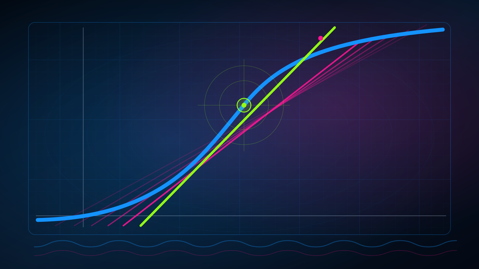
A secant line becomes a tangent line

FunctionSecantTangent

Approach from

LeftRight

Distance from the fixed point: |h| = 1.00

Secant slopem_h = 2 + (1.00) = 3.00Tangent slope: 2.00

The blue curve in the diagram is the graph of $f(x)=x^2$. A line through two points on that curve is a secant line. Its slope is an average rate of change. As the movable point approaches $(1,1)$, the secant lines approach a tangent line. The tangent line’s slope is the derivative at $x=1$.

The formal definition

Let $f$ be a function, and let $a$ be an input where we want to measure local change. The derivative of $f$ at $a$ is

$$f'(a)=\lim_{h\to 0}\frac{f(a+h)-f(a)}{h},$$

provided that the limit exists.

Each symbol has a specific job:

• $f(a)$ is the output at the fixed input $a$.
• $h$ is a nonzero horizontal offset.
• $f(a+h)-f(a)$ is the corresponding change in output.
• Dividing the output change by $h$ gives the slope between two points.
• Taking the limit asks whether those slopes approach one finite number as $h$ approaches zero from both sides.

A derivative need not exist everywhere. The graph of $f(x)=|x|$, for example, has a sharp corner at $x=0$. Secant slopes approach $-1$ from the left and $1$ from the right. Because the two sides disagree, no single tangent slope exists there.

Worked example: find a tangent line

Consider

$$f(x)=x^2+2x.$$

We will find the derivative at $x=3$ and then find the line tangent to the curve there.

First calculate the fixed output:

$$f(3)=3^2+2(3)=15.$$

Now apply the definition:

$$f'(3)=\lim_{h\to 0}\frac{f(3+h)-f(3)}{h}.$$

Expand $f(3+h)$ without skipping the middle terms:

$$\begin{aligned} f(3+h) &=(3+h)^2+2(3+h)\\ &=9+6h+h^2+6+2h\\ &=15+8h+h^2. \end{aligned}$$

Substitute that expression into the difference quotient:

$$\begin{aligned} f'(3) &=\lim_{h\to 0}\frac{15+8h+h^2-15}{h}\\ &=\lim_{h\to 0}\frac{8h+h^2}{h}\\ &=\lim_{h\to 0}(8+h)\\ &=8. \end{aligned}$$

The derivative supplies the tangent line’s slope, $8$. The curve passes through $(3,15)$, so the point-slope equation is

$$y-15=8(x-3).$$

Expanding the right side gives the tangent line

$$y=8x-9.$$

Try it yourself

Problem 1

For $f(x)=x^2$, find $f'(4)$ from the limit definition. Then find the tangent line at $x=4$.

Reveal the solution

Begin with $f(4)=16$:

$$\begin{aligned} f'(4) &=\lim_{h\to0}\frac{(4+h)^2-16}{h}\\ &=\lim_{h\to0}\frac{16+8h+h^2-16}{h}\\ &=\lim_{h\to0}(8+h)\\ &=8. \end{aligned}$$

The tangent line passes through $(4,16)$ with slope $8$:

$$y-16=8(x-4),$$

so $y=8x-16$.

Problem 2

An object’s position is $s(t)=5t^2+2t$ meters. Find its instantaneous velocity at $t=3$ seconds using the limit definition.

Reveal the solution

First, $s(3)=5(9)+6=51$ meters. Then

$$\begin{aligned} s'(3) &=\lim_{h\to0}\frac{5(3+h)^2+2(3+h)-51}{h}\\ &=\lim_{h\to0}\frac{45+30h+5h^2+6+2h-51}{h}\\ &=\lim_{h\to0}\frac{32h+5h^2}{h}\\ &=\lim_{h\to0}(32+5h)\\ &=32. \end{aligned}$$

The instantaneous velocity at $t=3$ is $32$ meters per second.

How the idea emerged

The derivative accumulated rather than arriving in one clean act of discovery.

During the seventeenth century, mathematicians were trying to solve several problems that turned out to share a hidden structure. How do you draw a tangent to a curve? How do you locate a maximum or minimum? How do you describe motion whose speed keeps changing? How do you recover distance from a changing velocity?

Pierre de Fermat developed a method for tangents, maxima, and minima before a general calculus existed. Evangelista Torricelli and Isaac Barrow studied variable-speed motion and the inverse relationship between finding velocity and recovering distance. The MacTutor history of calculus traces how these separate techniques began to converge.

Isaac Newton treated quantities as flowing through time and called their rates of change fluxions. His surviving October 1666 tract on fluxions records an early systematic version of the method, but Newton did not publish that tract at the time.

Gottfried Wilhelm Leibniz developed calculus from a different starting point during the 1670s. He emphasized symbolic differences such as $dx$ and $dy$, along with rules that could be reused across many problems. Leibniz published differential calculus in 1684, before Newton published a comparable account, and his notation became the dominant language of calculus.

This chronology produced one of mathematics’ ugliest credit disputes. Manuscripts, private correspondence, public articles, and institutional reputation all offered competing definitions of priority. The Royal Society eventually judged a dispute involving its own president, Newton. The Society’s archive notes that Brook Taylor served on its priority committee, while the Newton Project’s timeline records Newton’s extensive and sometimes anonymous role in defending the resulting report. The argument hardened a mathematical disagreement into rival British and Continental camps.

Modern histories credit Newton and Leibniz with independent, differently conceived systems while recognizing the work that Fermat, Barrow, Torricelli, and others had already done. The episode is also a warning about the politics of discovery: an institution can preserve knowledge and still be poorly positioned to arbitrate credit involving its own leader.

Neither Newton’s fluxions nor Leibniz’s infinitesimals had the modern logical foundation used in this lesson. Critics attacked the gaps. Nineteenth-century mathematicians, especially Augustin-Louis Cauchy and later Karl Weierstrass, helped recast derivatives in terms of limits precise enough to support modern analysis.

Where derivatives work

The derivative measures a local response. Change the labels on the two axes, and the same calculation answers questions in different fields.

Application map

One local slope, three different questions

Motion

The slope of position is instantaneous velocity.

Economics

The slope of total cost is marginal cost.

Machine learning

The slope identifies a direction that reduces loss.

For motion, differentiating position produces velocity; differentiating velocity produces acceleration. In economics, differentiating total cost with respect to production gives marginal cost, the local cost of producing a little more. In machine learning, models often adjust many parameters by following derivatives of a loss function. Google’s gradient descent explanation shows how repeated downhill steps can reduce that loss.

The one-dimensional derivative $f'(x)$ becomes a gradient when a function has many inputs. A gradient is a vector assembled from partial derivatives, one for each input. The concept is larger, but the local question survives: if this input changes slightly, how does the output respond?

Derivatives also support hypothetical applications wherever a future system must react to continuous change. An autonomous spacecraft could use local rates to revise a trajectory after a tiny thrust error. A climate-control system could estimate how quickly a building’s temperature responds to sunlight. The physical models would differ; both systems would need a disciplined answer to “what is changing here, and how fast?”

One idea to remember

A derivative does not divide zero by zero. It compares two distinct points, moves them arbitrarily close together, and asks whether their slopes settle toward one number.

That number is the best linear description of how a function is changing at one location. For a position function, we call it velocity. For a graph, we call it tangent slope. The mathematics underneath is the same reckoning.

The natural next lesson is the limit itself: what it means for values to approach a number, and how mathematicians make “arbitrarily close” exact.

Sources

• OpenStax, Calculus Volume 1: Defining the Derivative
• MacTutor History of Mathematics: The Rise of Calculus
• The Newton Project: The October 1666 Tract on Fluxions
• The Royal Society: Brook Taylor and the Newton–Leibniz Calculus Controversy
• The Newton Project: Isaac Newton’s Life and Work at a Glance
• Google for Developers: Gradient Descent