How Does Mathematics Make ‘Close’ Exact?

Enter numbers increasingly close to $2$ into the function $f(x)=x^2$:

Input $x$	Output $f(x)$
$1.9$	$3.61$
$1.99$	$3.9601$
$1.999$	$3.996001$

The outputs appear to approach $4$. A table can suggest that behavior, but no finite list can test every input near $2$. How could a proof cover infinitely many nearby inputs at once?

The answer is a challenge-and-response game. A challenger names any acceptable output error, however tiny. The proof responds with an input radius that guarantees the requested accuracy. The Greek letters epsilon, written $\varepsilon$, and delta, written $\delta$, traditionally name those two positive numbers.

A guarantee with two distances

First consider a specific challenge. Suppose we want $x^2$ to land within $0.5$ of $4$. Choosing $x$ within $0.1$ of $2$ works: the condition $1.9<x<2.1$ forces

$$3.61<x^2<4.41,$$

so $|x^2-4|<0.5$. Here the output tolerance is $\varepsilon=0.5$, and the input radius is $\delta=0.1$.

A limit proof must answer every positive tolerance, including tolerances far smaller than $0.5$. For $f(x)=x^2$, a dependable response is

$$\delta=\min\left(1,\frac{\varepsilon}{5}\right).$$

The notation $\min(u,v)$ means the smaller of the two numbers $u$ and $v$. The fixed choice $1$ keeps $x$ in a region where the curve cannot grow too steeply; the fraction $\varepsilon/5$ adjusts the input radius to the challenger’s requested accuracy.

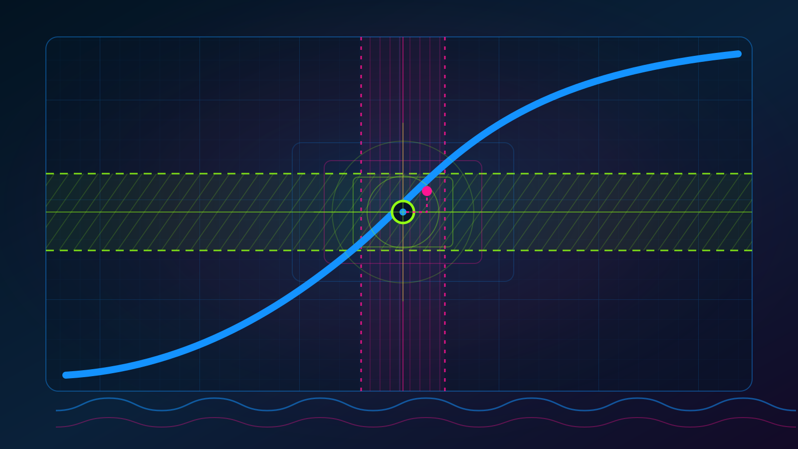
The interactive graph below shows both distances. The green horizontal band contains outputs within $\varepsilon$ of $4$. The magenta vertical corridor contains inputs within $\delta$ of $2$. Move the test point inside and outside the corridor, or tighten the tolerance. A striped boundary and geometric shape accompany each color cue.

Interactive diagram

Turn an output tolerance into an input tolerance

ε output bandδ input windowf(x) = x²

Choose the output tolerance: ε = 1Move the test point: x = 2.16

Inside δOutside δ

Proof's responseδ = min(1, ε/5) = 0.2

Input distance|x − 2| = 0.16

Output distance|x² − 4| = 0.666

Guarantee active: the point lies inside both tolerance windows.

The precise definition

Let $f$ be a function. Let $a$ be the input that nearby values approach, and let $L$ be the output that $f(x)$ appears to approach. We write

$$\lim_{x\to a}f(x)=L$$

when the following statement is true:

For every $\varepsilon>0$, there exists a $\delta>0$ such that, for every input $x$, if $0<|x-a|<\delta$, then $|f(x)-L|<\varepsilon$.

OpenStax gives this same precise definition and develops its geometric meaning. Every symbol in the statement measures something specific:

• $|f(x)-L|$ is the distance from the output $f(x)$ to the proposed limit $L$.
• $\varepsilon$ is the largest output error the challenger will accept.
• $|x-a|$ is the distance from the input $x$ to the approached input $a$.
• $\delta$ is the input radius supplied by the proof.
• The condition $0<|x-a|$ excludes $x=a$ itself.

The order of the words matters. The challenger chooses $\varepsilon$ first. The proof may choose $\delta$ after seeing $\varepsilon$, so $\delta$ may depend on $\varepsilon$, the function $f$, the input $a$, and the proposed limit $L$. The proof must then handle every $x$ in the punctured interval $0<|x-a|<\delta$; it cannot choose a different $\delta$ after seeing an inconvenient $x$.

Excluding the center lets a limit describe nearby behavior even when the function has a hole or an unusual value there. Define

$$g(x)= \begin{cases} x^2, & x\ne 2,\\ 100, & x=2. \end{cases}$$

Although $g(2)=100$, every nearby value $g(x)$ with $x\ne2$ equals $x^2$. Therefore

$$\lim_{x\to2}g(x)=4.$$

A limit records where nearby outputs go. It does not, by itself, dictate the output at the approached input.

Worked example: prove that $x^2$ approaches $4$

We will prove

$$\lim_{x\to2}x^2=4.$$

Begin with an arbitrary number $\varepsilon>0$. We need to find a positive $\delta$ that turns $0<|x-2|<\delta$ into $|x^2-4|<\varepsilon$.

Factoring the output error reveals two factors:

$$|x^2-4|=|(x-2)(x+2)|=|x-2|\,|x+2|.$$

The first factor is exactly the input distance that we can control. To control the second factor, require $\delta\le1$. Then $|x-2|<\delta\le1$ implies

$$-1<x-2<1,$$

and adding $2$ to all three parts gives

$$1<x<3.$$

Adding $2$ again yields $3<x+2<5$, so $|x+2|<5$. Now choose

$$\delta=\min\left(1,\frac{\varepsilon}{5}\right).$$

This choice is positive because $\varepsilon>0$. If $0<|x-2|<\delta$, then the earlier bound $|x+2|<5$ applies, and

$$\begin{aligned} |x^2-4| &=|x-2|\,|x+2|\\ &<5|x-2|\\ &<5\delta\\ &\le5\left(\frac{\varepsilon}{5}\right)\\ &=\varepsilon. \end{aligned}$$

The final inequality uses $\delta\le\varepsilon/5$, which follows from the definition of $\min$. Because the argument works for every positive $\varepsilon$, the limit is proved.

The response $\delta=\min(1,\varepsilon/5)$ is sufficient rather than uniquely best. A smaller positive radius would also work. Epsilon–delta proofs ask for a guarantee, not the widest possible interval.

Try the challenge

Problem 1

Use the epsilon–delta definition to prove

$$\lim_{x\to3}(2x+1)=7.$$

Reveal the solution

Let $\varepsilon>0$ be arbitrary. The output error is

$$|(2x+1)-7|=|2x-6|=2|x-3|.$$

Choose $\delta=\varepsilon/2$. This number is positive. If $0<|x-3|<\delta$, then

$$|(2x+1)-7|=2|x-3|<2\delta=2\left(\frac{\varepsilon}{2}\right)=\varepsilon.$$

Therefore $\lim_{x\to3}(2x+1)=7$.

Problem 2

Use the epsilon–delta definition to prove

$$\lim_{x\to3}x^2=9.$$

Reveal the solution

Let $\varepsilon>0$ be arbitrary. Factor the output error:

$$|x^2-9|=|x-3|\,|x+3|.$$

Choose

$$\delta=\min\left(1,\frac{\varepsilon}{7}\right).$$

If $0<|x-3|<\delta$, then $|x-3|<1$, so $2<x<4$. Consequently, $5<x+3<7$ and $|x+3|<7$. Therefore

$$\begin{aligned} |x^2-9| &=|x-3|\,|x+3|\\ &<7|x-3|\\ &<7\delta\\ &\le7\left(\frac{\varepsilon}{7}\right)\\ &=\varepsilon. \end{aligned}$$

The argument proves $\lim_{x\to3}x^2=9$.

How “as close as desired” became mathematics

The modern definition did not appear in one person’s notebook on one date. It emerged as mathematicians tried to replace persuasive geometric pictures and infinitesimal quantities with statements that could survive every exceptional case.

In 1817, the Prague mathematician and philosopher Bernard Bolzano published a “purely analytic” proof of a theorem about continuous functions. His work pursued rigor without relying on geometric intuition, but it circulated poorly and was probably unknown to the mathematicians who soon made similar advances. The MacTutor biography of Bolzano places his mathematics inside Habsburg rule in Bohemia: after Bolzano advocated pacifism, social equality, and intellectual freedom, the Austrian government removed him from his university post in 1819, censored his mail, and restricted his publication.

Augustin-Louis Cauchy’s 1821 textbook Cours d’analyse defined a limit in verbal terms, through variable values approaching a fixed value without end. A public-domain scan of the 1821 book preserves the primary text. Cauchy used both $\varepsilon$ and $\delta$ in an 1823 proof, although he did not yet express their dependency with the modern quantifier structure. Karl Weierstrass systematized that structure in his 1861 lectures. Historian G. I. Sinkevich traces the transition from verbal limits to full “epsilontics”, while Judith V. Grabiner’s study reconstructs the longer route to Cauchy’s rigorous calculus.

Politics touched Cauchy’s career too. He gained an Académie des Sciences seat in 1816 after the restored Bourbon government removed Lazare Carnot and Gaspard Monge. Following the July Revolution of 1830, Cauchy refused to swear allegiance to the new regime and lost academic posts that required the oath. The MacTutor biography of Cauchy documents both turns. Bolzano’s suppression and Cauchy’s shifting access to institutions did not determine whether their proofs were correct. Those events did affect careers, audiences, and which work traveled easily enough to be read.

Where exact tolerances matter

Epsilon–delta language anchors the modern theory of continuity, derivatives, and integrals. The same pattern also appears whenever a calculation must meet a declared error budget: state the permitted output error, then determine what accuracy the inputs or intermediate steps require.

Numerical simulation software uses this pattern operationally. An adaptive time-stepping program estimates the error produced by one simulated step and compares that estimate with a specified tolerance. The program accepts, rejects, or resizes the step in response. The National Institute of Standards and Technology guide to numerical implementation describes that error-control loop.

Iterative algorithms create a sequence of improving approximations. For example, Newton’s method estimates $\sqrt2$ by starting with a positive number $x_0$ and repeatedly calculating

$$x_{n+1}=\frac12\left(x_n+\frac{2}{x_n}\right),$$

where $n$ counts completed steps. Starting from $x_0=1.5$, three repetitions produce an estimate whose error is about $1.6\times10^{-12}$. The four number lines below use a different scale in each row, so each row can show both the current estimate and a much tighter permitted error.

Numerical convergence

Each calculation earns a tighter error budget

Production solvers turn the visual idea into a stopping rule. For example, the National Institute of Standards and Technology documentation for a conjugate-gradient solver describes repeated approximations that stop when a relative error falls below a chosen tolerance.

Speculative application: a future formally verified artificial-intelligence controller could attach mathematical error certificates to decisions made near a safety boundary. Such a certificate might guarantee that sensor uncertainty below a computed $\delta$ changes a risk score by less than a regulator’s chosen $\varepsilon$. Building a trustworthy physical model would remain the hard part; epsilon–delta reasoning would supply the form of the guarantee.

One idea to remember

To prove that $f(x)$ approaches $L$ as $x$ approaches $a$, accept every positive output tolerance $\varepsilon$ and answer it with a positive input radius $\delta$ that works for every nearby $x$.

Yesterday’s Reckoning, “How Can Motion Have a Speed at One Instant?”, used a limit to define instantaneous velocity. Today’s guarantee supplies the missing logical machinery. Natural directions from here are continuity, which asks whether a function’s value agrees with its limit, and sequential limits, which test approach using every convergent sequence of inputs.

Sources

• OpenStax, Calculus Volume 1: The Precise Definition of a Limit
• MacTutor History of Mathematics: Bernard Bolzano
• Augustin-Louis Cauchy, Cours d’analyse (1821), Internet Archive
• G. I. Sinkevich, “On the History of Epsilontics”
• Judith V. Grabiner, “Who Gave You the Epsilon?”
• MacTutor History of Mathematics: Augustin-Louis Cauchy
• National Institute of Standards and Technology: Numerical Implementation Guide
• National Institute of Standards and Technology: Conjugate Gradient Solver