Can a Random Process Forget Where It Started?

Suppose tomorrow’s weather depends on today’s weather according to two rules:

• After a sunny day, the next day is sunny with probability 80% and rainy with probability 20%.
• After a rainy day, the next day is sunny with probability 40% and rainy with probability 60%.

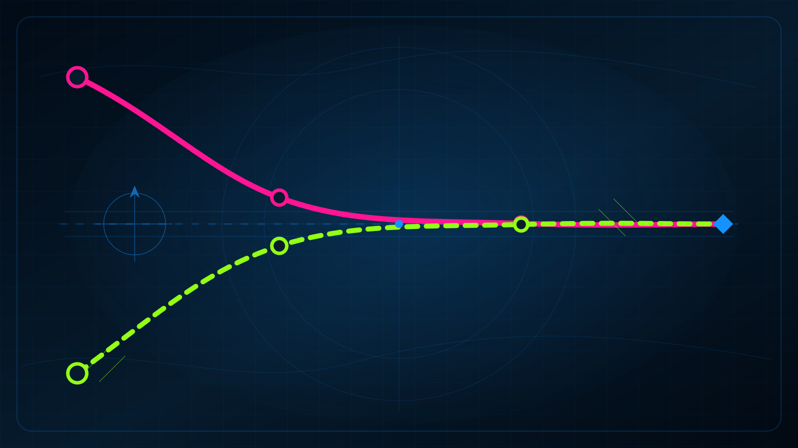
Now place two forecasters in different rooms. One knows that day zero was sunny. The other knows that day zero was rainy. Neither forecaster receives another observation. They use the same two rules to predict each later day.

Will their forecasts ever agree?

They will not become exactly equal after any finite number of days. Their disagreement will shrink by 60% every day, however, and both forecasts will approach the same answer: a $\frac{2}{3}$ chance of sun. The process remembers the present while gradually losing information about its beginning.

A chain with one-step memory

Let $X_n$ name the weather on day $n$. Each $X_n$ can have one of two states, sunny or rainy. This weather model is a Markov chain because the probabilities for day $n+1$ depend on the state at day $n$, not on the complete sequence of earlier states.

The Markov property can be written precisely as

$$\Pr(X_{n+1}=j\mid X_n=i,X_{n-1},\ldots,X_0) = \Pr(X_{n+1}=j\mid X_n=i).$$

Here $\Pr$ means probability; $i$ is the current state; $j$ is a possible next state; and the vertical bar means “given that.” The equation says that once the current state $X_n=i$ is known, earlier states add no information about the next step.

That condition is a claim about a mathematical model, not a law that every real weather system obeys. An actual forecast uses atmospheric measurements and far more than one day of history. The two-state chain is small enough to expose the mathematics.

We can collect the four transition probabilities in a table called a transition matrix:

$$P= \begin{pmatrix} 0.8 & 0.2\\ 0.4 & 0.6 \end{pmatrix}.$$

The rows describe today’s state in the order sunny, rainy. The columns describe tomorrow’s state in the same order. Every row sums to $1$ because tomorrow must be either sunny or rainy.

The diagram below first shows those four transitions. Its graph then follows two forecasts—one beginning with certain sun, the other with certain rain. Advance the day and watch the vertical gap.

Interactive probability forecast

Two forecasts forget two different beginnings

Day 0

Started sunny: 100.00%

Same transition rules

Started rainy: 0.00%

Gap: 100.00 percentage points

Advance one dayReset

One number is enough for two states

Let $p_n$ be the probability of sun on day $n$. The probability of rain is then $1-p_n$, so a separate variable is unnecessary.

Tomorrow can be sunny by either of two routes:

1. Today is sunny, with probability $p_n$, and sun persists, with probability $0.8$.
2. Today is rainy, with probability $1-p_n$, and rain changes to sun, with probability $0.4$.

Add the probabilities of those mutually exclusive routes:

$$\begin{aligned} p_{n+1} &=0.8p_n+0.4(1-p_n)\\ &=0.8p_n+0.4-0.4p_n\\ &=0.4+0.4p_n. \end{aligned}$$

The last line is the whole forecasting machine.

Worked example: begin with certain sun

If day zero is known to be sunny, then $p_0=1$. Apply the recurrence one day at a time:

$$\begin{aligned} p_1&=0.4+0.4(1)=0.8,\\ p_2&=0.4+0.4(0.8)=0.72,\\ p_3&=0.4+0.4(0.72)=0.688,\\ p_4&=0.4+0.4(0.688)=0.6752. \end{aligned}$$

The probability of sun moves from 100% to 80%, then 72%, 68.8%, and 67.52%. The changes become smaller because the forecast is approaching a value that the update rule leaves unchanged.

Call that unchanged probability $p_*$. It must satisfy

$$\begin{aligned} p_*&=0.4+0.4p_*\\ p_*-0.4p_*&=0.4\\ 0.6p_*&=0.4\\ p_*&=\frac{0.4}{0.6}=\frac{2}{3}. \end{aligned}$$

The full long-run distribution is therefore

$$\boldsymbol{\pi}=\left(\frac{2}{3},\frac{1}{3}\right),$$

where the first coordinate is the probability of sun and the second is the probability of rain. A probability distribution $\boldsymbol{\pi}$ is stationary for a transition matrix $P$ when

$$\boldsymbol{\pi}P=\boldsymbol{\pi}.$$

Starting with $\boldsymbol{\pi}$ and applying one more transition changes nothing.

Why the beginning fades

Subtract the equilibrium probability $\frac{2}{3}$ from both sides of the recurrence:

$$\begin{aligned} p_{n+1}-\frac{2}{3} &=0.4+0.4p_n-\frac{2}{3}\\ &=0.4\left(p_n-\frac{2}{3}\right). \end{aligned}$$

The distance from equilibrium is multiplied by $0.4$ each day. After $n$ days,

$$p_n-\frac{2}{3}=0.4^n\left(p_0-\frac{2}{3}\right).$$

Since $0.4^n$ approaches zero as $n$ grows, the effect of the starting probability $p_0$ disappears. This shrinking factor also explains the graph: the gap between the two forecasts is $1$ on day zero, $0.4$ on day one, $0.16$ on day two, and $0.064$ on day three.

Not every Markov chain forgets. A rule that alternates between sun and rain with 100% certainty oscillates forever. A process with two states that can never leave once entered remembers its initial state forever. For finite chains, convergence to one stationary distribution is guaranteed under conditions commonly called irreducibility—every state can eventually reach every other state—and aperiodicity, which rules out forced rhythmic cycles. Stanford’s notes on mixing times state those conditions precisely. Our weather chain satisfies both because all four one-step transition probabilities are positive.

Try the update rule

Problem 1

Begin with a rainy day, so $p_0=0$. What is the probability of sun on day two?

Reveal the solution

Apply $p_{n+1}=0.4+0.4p_n$ twice:

$$\begin{aligned} p_1&=0.4+0.4(0)=0.4,\\ p_2&=0.4+0.4(0.4)=0.56. \end{aligned}$$

The probability of sun on day two is 56%.

Problem 2

Change the rules: sun persists with probability 70%, while rain changes to sun with probability 20%. Find the stationary probability of sun.

Reveal the solution

If $p$ is the current probability of sun, the next probability is

$$0.7p+0.2(1-p)=0.2+0.5p.$$

At stationarity, the next probability equals the current probability $p_*$:

$$\begin{aligned} p_*&=0.2+0.5p_*\\ 0.5p_*&=0.2\\ p_*&=0.4. \end{aligned}$$

The stationary probability of sun is 40%. The stationary probability of rain is 60%.

A mathematical argument about free will

Andrey Markov developed the first general theory of chains of dependent events in a 1906 paper. His target was not weather. It was a claim made by another Russian mathematician, Pavel Nekrasov, about probability, society, and free will.

Nekrasov argued in 1902 that the law of large numbers required independent events. He then treated human voluntary acts as independent and used stable social statistics, including crime statistics, to support a theological account of free will. Markov objected to the mathematics. He constructed dependent random sequences that still obeyed a law of large numbers, removing the step on which Nekrasov’s philosophical argument depended.

The disagreement belonged to a wider political divide in late-imperial Russia. Markov was a secular republican in St. Petersburg; Nekrasov was an ecclesiastical monarchist at Moscow University, then closely tied to the Russian Orthodox Church. Markov also protested Tsar Nicholas II’s veto of the writer Maxim Gorky’s election to the Imperial Academy of Sciences and asked the Church to excommunicate him after it excommunicated Leo Tolstoy. Brian Hayes reconstructs this collision of mathematics, politics, and theology in First Links in the Markov Chain, drawing on historian Eugene Seneta’s research.

Markov’s 1906 theory was abstract. In 1913 he gave it a memorable body: the first 20,000 letters of Alexander Pushkin’s verse novel Eugene Onegin. Markov classified each letter as a vowel or consonant and counted how often one type followed the other. The letters were dependent—vowels and consonants alternated more often than independence would predict. The published English translation of that 1913 study did not appear until 2006, a delay traced in the same historical account.

Markov did not invent his chains to imitate prose. Pushkin’s poem supplied concrete evidence that dependent events could be analyzed with exact probability.

Where the same idea works now

A web surfer’s current page influences which page comes next. Sergey Brin and Lawrence Page used that structure in PageRank, assigning importance through repeated movement across the web’s link graph. Their 1998 description of the early Google search engine explains how link structure produced a ranking for each page. In the Markov-chain interpretation developed in later Stanford research, the ranking is a stationary distribution: pages visited often by the long-running random surfer receive more weight.

In biology, the true state of a DNA segment—such as whether it belongs to a gene—may be hidden while its nucleotide sequence is visible. Hidden Markov models add observations to unobserved states and use transition probabilities to infer likely biological structure. A peer-reviewed tutorial review in Current Genomics surveys uses in gene prediction, sequence alignment, and protein modeling.

Markov chains also let computers sample from distributions that are too large to list directly. A program designs transitions so that the desired distribution is stationary, runs the chain long enough to reduce the influence of its starting point, and keeps the resulting states as approximate samples. That family of methods is called Markov chain Monte Carlo. Stanford’s algorithm notes show how the same stationary-distribution idea becomes a sampling scheme.

Every application inherits the warning from our weather toy: a stationary distribution is useful only if the chain actually approaches it fast enough. “Eventually” can be mathematically true and computationally useless.

One idea to remember

A Markov chain uses the present state to choose the next one. When its transitions mix rather than trap or force a cycle, repeated updates can erase the starting state and approach a stationary distribution.

To continue, investigate transition matrices, eigenvectors, and mixing time—the number of steps required before the remaining memory is smaller than a chosen tolerance.

Sources

• Brian Hayes, “First Links in the Markov Chain,” American Scientist 101(2), 2013.
• Eugene Seneta, “Markov and the Birth of Chain Dependence Theory,” International Statistical Review 64(3), 1996.
• Stanford University, “Mixing Times,” CS265/CME309 lecture notes.
• Sergey Brin and Lawrence Page, “The Anatomy of a Large-Scale Hypertextual Web Search Engine,” 1998.
• Sepandar Kamvar, Taher Haveliwala, and Gene Golub, “Adaptive Methods for the Computation of PageRank,” 2004.
• Byung-Jun Yoon, “Hidden Markov Models and their Applications in Biological Sequence Analysis,” Current Genomics 10(6), 2009.
• Tim Roughgarden and Gregory Valiant, “Markov Chain Monte Carlo,” Stanford CS168, 2024.