How Can Smooth Waves Build a Square Wave?

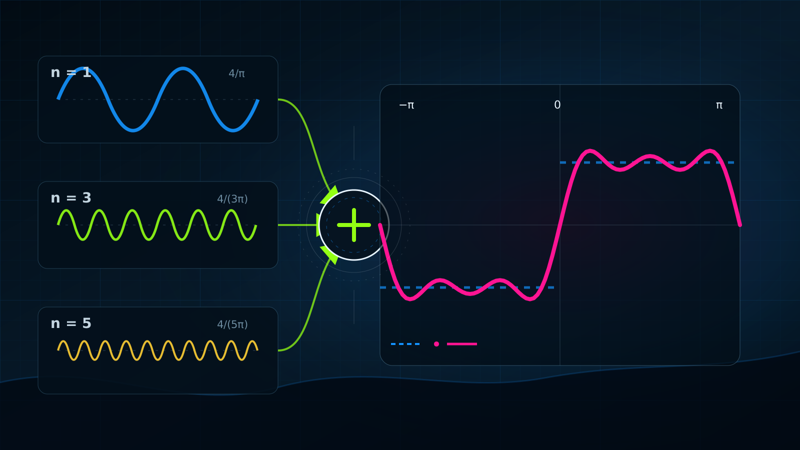
A sine wave bends everywhere. A square wave stays flat, then jumps in an instant. How could any pile of smooth sine waves produce a shape with corners and vertical cliffs?

No finite pile succeeds exactly. Yet an infinite sequence of carefully weighted sine waves reproduces every flat stretch of a square wave and converges to a precise compromise at each jump. The first few waves already make the construction visible.

Give the target a definition

Let $q(x)$ denote a square wave on the interval from $-\pi$ to $\pi$. Define it by

$$q(x)= \begin{cases} -1, & -\pi<x<0,\\ 0, & x=0,\\ 1, & 0<x<\pi. \end{cases}$$

Then repeat the same shape every $2\pi$ units, so $q(x+2\pi)=q(x)$. The symbol $x$ marks horizontal position, and $\pi$ radians is half of one full cycle. At the repeated jump points, including $0$ and $\pi$, assign the value halfway between the two plateaus: $0$.

The interactive figure below begins with three sine waves. Move the slider from one harmonic to fifteen. The upper plot shows their sum; the lower plot shows the coefficient attached to each frequency.

Harmonic builder

Add smooth waves and watch corners appear

Reset to 3 harmonics

Odd harmonics included

3

Terms used3 odd harmonics

Highest frequency5 × fundamental

Value at x = π/21.103

The recipe uses only odd harmonics

Bar height is the coefficient 4 / (πn).

The curve acquires flatter decks and steeper sides because the added sine waves oscillate faster. Their amplitudes shrink at the same time. The first frequency supplies the broad outline, while each later frequency corrects smaller-scale error.

The frequency recipe

For every $x$ that is not a jump point, the square wave has the Fourier series

$$q(x)=\frac{4}{\pi} \sum_{k=0}^{\infty} \frac{\sin\big((2k+1)x\big)}{2k+1}.$$

The index $k$ runs through the nonnegative integers $0,1,2,\ldots$. Therefore $2k+1$ runs through the odd harmonic numbers $1,3,5,\ldots$. The word harmonic means an integer multiple of the base frequency. Writing out the first terms gives

$$q(x)=\frac{4}{\pi} \left( \sin x+\frac{\sin 3x}{3}+\frac{\sin 5x}{5}+\frac{\sin 7x}{7}+\cdots \right).$$

The equality describes the infinite series. A graph on a screen can only draw a partial sum. Using the first $N$ odd harmonics gives

$$S_N(x)=\frac{4}{\pi} \sum_{k=0}^{N-1} \frac{\sin\big((2k+1)x\big)}{2k+1},$$

where $N$ is the number of included sine waves. The interactive figure draws $S_N(x)$.

Why the even harmonics vanish

A general $2\pi$-periodic Fourier series can contain a constant, cosine waves, and sine waves. The coefficient of $\sin(nx)$ is

$$b_n=\frac{1}{\pi}\int_{-\pi}^{\pi}q(x)\sin(nx)\,dx,$$

where $n$ is a positive integer. The square wave $q(x)$ and the sine wave $\sin(nx)$ both change sign when $x$ changes sign. Their product does not change sign, so the product is symmetric about $0$. We may double the integral over the positive half:

$$\begin{aligned} b_n &=\frac{2}{\pi}\int_0^{\pi}\sin(nx)\,dx\\ &=\frac{2}{\pi}\left[-\frac{\cos(nx)}{n}\right]_0^{\pi}\\ &=\frac{2}{\pi n}\bigl(1-\cos(n\pi)\bigr)\\ &=\frac{2}{\pi n}\bigl(1-(-1)^n\bigr). \end{aligned}$$

When $n$ is even, $(-1)^n=1$, so $b_n=0$. When $n$ is odd, $(-1)^n=-1$, so

$$b_n=\frac{4}{\pi n}.$$

That calculation produces the descending odd bars in the lower diagram. The constant and every cosine coefficient are also $0$ because the square wave is odd: $q(-x)=-q(x)$. A constant or cosine term would introduce an even component that the waveform does not have.

Worked example: three harmonics at the middle of a plateau

Evaluate the three-term approximation $S_3(x)$ at $x=\pi/2$. Begin with the definition:

$$S_3\left(\frac{\pi}{2}\right) =\frac{4}{\pi} \left( \sin\frac{\pi}{2} +\frac{1}{3}\sin\frac{3\pi}{2} +\frac{1}{5}\sin\frac{5\pi}{2} \right).$$

The three sine values are $1$, $-1$, and $1$. Substitute them one at a time:

$$\begin{aligned} S_3\left(\frac{\pi}{2}\right) &=\frac{4}{\pi}\left(1-\frac13+\frac15\right)\\ &=\frac{4}{\pi}\left(\frac{15-5+3}{15}\right)\\ &=\frac{4}{\pi}\cdot\frac{13}{15}\\ &=\frac{52}{15\pi}\\ &\approx1.103. \end{aligned}$$

The target value is $q(\pi/2)=1$, so three harmonics overshoot by about $0.103$ there. More terms make the middle of the plateau settle toward $1$.

Near a jump, the behavior is stranger. The tallest overshoot approaches about $1.179$ even as more terms are added. Its height does not fall to $1$; instead, the overshooting region becomes narrower. This persistent ringing is called the Gibbs phenomenon. At the jump itself, every term contains $\sin(0)=0$, so every partial sum equals $0$—the average of the neighboring values $-1$ and $1$. MIT OpenCourseWare’s notes on the standard square wave derive the same coefficients and describe this midpoint rule at discontinuities.

Try two checks

Problem 1

Use only the first two odd harmonics. What is $S_2(\pi/2)$?

Reveal the solution

The two-term partial sum is

$$S_2(x)=\frac{4}{\pi}\left(\sin x+\frac{\sin3x}{3}\right).$$

At $x=\pi/2$, the two sine values are $1$ and $-1$:

$$\begin{aligned} S_2\left(\frac{\pi}{2}\right) &=\frac{4}{\pi}\left(1-\frac13\right)\\ &=\frac{4}{\pi}\cdot\frac23\\ &=\frac{8}{3\pi}\\ &\approx0.849. \end{aligned}$$

The second harmonic correction leaves the approximation below the plateau. Adding the next odd harmonic raises it above the plateau to about $1.103$.

Problem 2

What is $S_N(0)$ for any positive whole number $N$? Explain without adding the terms individually.

Reveal the solution

Every term in the partial sum has the form

$$\frac{4}{\pi}\cdot\frac{\sin((2k+1)x)}{2k+1}.$$

At $x=0$,

$$\sin((2k+1)\cdot0)=\sin0=0$$

for every value of $k$. A sum of zeros is zero, so

$$S_N(0)=0$$

for every positive whole number $N$. The Fourier series lands exactly halfway between the square wave’s left-hand value $-1$ and right-hand value $1$.

Heat, revolution, empire, and an unwelcome kind of function

Joseph Fourier did not begin with electronic signals. He wanted to calculate how heat spreads through a solid. Eighteenth-century mathematicians including Jean le Rond d’Alembert, Leonhard Euler, and Daniel Bernoulli had already argued about trigonometric sums while studying vibrating strings. Fourier pushed the idea into a broader claim: temperature profiles, including piecewise-defined profiles, could be decomposed into trigonometric waves and evolved one frequency at a time.

The mathematics emerged inside a life repeatedly redirected by political power. According to the University of St Andrews’ history of Fourier, he joined a local Revolutionary Committee in 1793, was imprisoned during the French Revolution, and escaped a possible death sentence after Robespierre’s fall. In 1798 Fourier joined Napoleon’s invasion of Egypt as a scientific adviser and became secretary of the Cairo Institute created during the French occupation. After Fourier returned to France, Napoleon appointed him prefect of the Isère department. Fourier began his sustained work on heat in Grenoble around 1804 while also serving as an imperial administrator.

Fourier presented a heat memoir to the Paris Institute in 1807. A committee that included Joseph-Louis Lagrange and Pierre-Simon Laplace objected to the trigonometric expansions and to parts of the physical derivation. A revised submission won the Institute’s 1811 prize, but the report still questioned its generality and rigor. Fourier’s Théorie analytique de la chaleur finally appeared in 1822.

That chronology resists a tidy discovery myth. Fourier did not invent trigonometric decomposition from nothing, and his original generality needed later mathematicians to state accurate convergence conditions. His decisive move was to treat a complicated temperature profile as a spectrum of frequencies and then solve the heat problem frequency by frequency. France’s revolutionary upheaval, a colonial military invasion, imperial administration, and the Paris Institute’s prize process all shaped Fourier’s working life and the route to publication. None of those facts proves that Fourier’s politics caused the series formula.

Where the frequency recipe works now

Heat and other diffusion problems. Fourier’s original method turns a starting temperature profile into sine and cosine modes. Each mode decays at its own rate, allowing a complicated cooling pattern to be calculated from elementary pieces.

Sound, communications, and electronics. Frequency components explain why two instruments playing the same note can sound different and how a filter changes a signal. MIT’s Signals and Systems materials use Fourier decomposition to show how a linear time-invariant system changes each harmonic’s amplitude and phase. A digital circuit’s near-square voltage contains the same odd-harmonic structure drawn above.

Images and magnetic resonance imaging. Two-dimensional Fourier methods encode spatial patterns as combinations of horizontal and vertical frequencies. The U.S. Food and Drug Administration’s magnetic resonance imaging test toolkit generates test data in the Fourier domain and reconstructs images from k-space with an inverse Fourier transform. Digital image processing uses the discrete version of the same frequency viewpoint; MIT’s discrete-time Fourier lecture connects the fast Fourier transform with image examples.

One idea to remember

A complicated periodic shape can be stored as a list of frequencies and weights. For the square wave, odd sine waves carry the entire recipe: frequency rises as $1,3,5,\ldots$, while amplitude falls as $1,1/3,1/5,\ldots$.

To continue, revisit how mathematics makes convergence exact or compare Fourier’s heat problem with the force balance behind a hanging chain. A later Reckoning can ask the next question: how does the Fourier transform extend the same idea from repeating signals to signals that never repeat?

Sources

• Joseph Fourier, Théorie analytique de la chaleur, Paris: Firmin Didot, 1822.
• University of St Andrews, “Joseph Fourier (1768–1830)”, MacTutor History of Mathematics, on Fourier’s mathematical, political, and administrative life.
• University of St Andrews, “Mathematicians and Music”, MacTutor History of Mathematics, on the vibrating-string debates preceding Fourier.
• Massachusetts Institute of Technology OpenCourseWare, “Fourier Series II”, 18.03 Differential Equations, Spring 2010.
• Massachusetts Institute of Technology OpenCourseWare, “Fourier Representations” and “Discrete-Time Fourier Representations”, 6.003 Signals and Systems, Fall 2011.
• U.S. Food and Drug Administration, “MRI-IQ-ETK: Digital MRI Test Phantoms and Automated Image Quality Evaluation Toolkit”, accessed September 14, 2026.