Why Do Averages Keep Drawing Bell Curves?

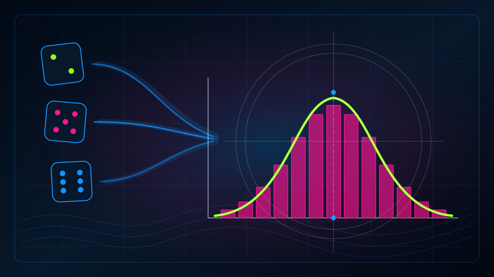
Roll one fair six-sided die. Its six results are equally likely, so its probability graph is flat, not bell-shaped.

Now roll several fair dice and record their average. An average near $3.5$ can be assembled in many ways: a low roll can balance a high roll, and countless mixed groups land near the middle. An average of exactly $1$, by contrast, requires every die to show $1$. The extreme outcomes run out of routes.

That imbalance in the number of routes is the seed of a bell curve.

Count every route

The diagram below does not run a random simulation. It counts all $6^n$ ordered results when $n$ fair dice are averaged. Select one, two, four, or eight dice. The bars show the exact distribution of the resulting average; the dashed curve is a normal distribution with the same center and spread.

Exact distribution explorer

Average more dice; watch the shape change

1 die2 dice4 dice8 dice

Average of4 dice

Center3.500

Standard error0.854

Exact outcomes counted1,296

The flat one-die graph is the starting population. The rounded graphs belong to sample averages, not to individual die rolls. That distinction is the central limit theorem’s actual subject.

Two changes happen as the number of dice grows:

1. The exact bars form a smoother, more symmetric mound around $3.5$.
2. The mound narrows because an average cancels some of the variation among individual rolls.

The bars never become a continuous curve. A finite group of dice can produce only finitely many averages. The dashed curve becomes a useful approximation to those discrete bars.

The theorem, stated precisely

Let $X_1,X_2,\ldots,X_n$ be independent random variables drawn from the same probability distribution. Suppose each variable has mean $\mu$ and finite, positive variance $\sigma^2$. The sample mean of the first $n$ variables is

$$\bar X_n=\frac{X_1+X_2+\cdots+X_n}{n}.$$

The classical central limit theorem says that the standardized variable

$$Z_n=\frac{\sqrt n\,(\bar X_n-\mu)}{\sigma}$$

converges in distribution to a standard normal random variable as $n$ grows. A standard normal random variable has mean $0$, variance $1$, and the familiar bell-shaped density

$$\phi(z)=\frac{1}{\sqrt{2\pi}}e^{-z^2/2}.$$

“Converges in distribution” means that probabilities for intervals under $Z_n$ approach the corresponding areas under the standard normal curve. It does not mean that every finite sample mean becomes literally normal.

The mean and variance of the unstandardized average are

$$\operatorname E[\bar X_n]=\mu, \qquad \operatorname{Var}(\bar X_n)=\frac{\sigma^2}{n}.$$

The standard deviation of $\bar X_n$ is therefore $\sigma/\sqrt n$. Statisticians call that quantity the standard error of the mean. The factor $1/\sqrt n$ explains why the diagram’s mound tightens while remaining centered at $3.5$.

Worked example: two dice make a triangle

Let $X_1$ and $X_2$ be two independent fair die rolls. Their average is

$$\bar X_2=\frac{X_1+X_2}{2}.$$

There are $6\times6=36$ equally likely ordered pairs. Count the pairs by their sum:

$$\begin{array}{c|rrrrrrrrrrr} X_1+X_2&2&3&4&5&6&7&8&9&10&11&12\\ \hline \text{number of pairs}&1&2&3&4&5&6&5&4&3&2&1 \end{array}$$

Dividing each sum by $2$ changes the horizontal labels but not the counts. The possible averages run from $1$ to $6$ in half-unit steps. The middle average, $3.5$, occurs when the sum is $7$:

$$(1,6),(2,5),(3,4),(4,3),(5,2),(6,1).$$

Thus

$$\Pr(\bar X_2=3.5)=\frac{6}{36}=\frac16.$$

The extreme average $1$ has only one route, $(1,1)$, so

$$\Pr(\bar X_2=1)=\frac{1}{36}.$$

One flat distribution convolved with another has produced a triangle. Repeating the same counting operation rounds the corners.

For one fair die,

$$\mu=\frac{1+2+3+4+5+6}{6}=\frac72=3.5.$$

Its second moment is

$$\operatorname E[X^2]=\frac{1^2+2^2+3^2+4^2+5^2+6^2}{6}=\frac{91}{6}.$$

Therefore its variance is

$$\sigma^2=\operatorname E[X^2]-\mu^2 =\frac{91}{6}-\left(\frac72\right)^2 =\frac{35}{12}.$$

For the average of four dice, the standard error is

$$\frac{\sigma}{\sqrt4} =\sqrt{\frac{35}{48}} \approx 0.854,$$

which matches the diagram’s readout.

Two problems to try

Problem 1

Two fair dice are averaged. What is the exact probability that their average equals $4$?

Reveal the solution

An average of $4$ means the sum is $8$. The ordered pairs are

$$(2,6),(3,5),(4,4),(5,3),(6,2).$$

Five of the $36$ equally likely pairs work, so

$$\Pr(\bar X_2=4)=\frac{5}{36}.$$

Problem 2

The standard deviation of one fair die is $\sqrt{35/12}$. What is the standard error of the average of nine independent fair dice?

Reveal the solution

Use the standard-error formula $\sigma/\sqrt n$ with $n=9$:

$$\frac{\sqrt{35/12}}{\sqrt9} =\frac{\sqrt{35/12}}{3} =\sqrt{\frac{35}{108}} \approx 0.569.$$

The average of nine dice has one third the standard deviation of one die.

A theorem assembled across centuries

The bell curve did not arrive as one person’s finished theorem. Abraham de Moivre found its earliest recognizable limit case while studying repeated games of chance. His 1733 pamphlet used a normal-shaped curve to approximate the number of heads in many fair coin tosses; the result entered the 1738 edition of The Doctrine of Chances. The University of St Andrews biography notes that de Moivre was a French Protestant who fled persecution after Louis XIV revoked the Edict of Nantes. In London, prejudice against foreigners helped keep him outside a university post, so he earned most of his income tutoring in homes and coffeehouses even after election to the Royal Society.

Pierre-Simon Laplace extended the approximation far beyond fair coins, culminating in his 1812 Théorie analytique des probabilités. During the nineteenth century, work by mathematicians including Siméon Denis Poisson, Pafnuty Chebyshev, and Andrey Markov broadened and sharpened the argument. Aleksandr Lyapunov supplied a general proof under explicit conditions in 1901. George Pólya coined the name central limit theorem in a 1920 paper. Vladimir Ulyanov’s historical review of classical and modern central limit theorems traces that progression and the later variants needed when the classical assumptions change.

The practical pressures also changed. Games of chance were an early source of questions, but probability became useful for annuities, mortality tables, astronomical errors, and repeated physical measurements. De Moivre himself published on life annuities, tying probability to the growing financial institutions that priced long-lived contracts.

Why the theorem matters—and where it stops

The theorem explains why uncertainty in a sample average is often approximated with a normal curve. That approximation underlies standard errors and many confidence intervals. The United States National Institute of Standards and Technology defines a standard error as the standard deviation of a statistic’s sampling distribution and notes the common approximate interval of two standard errors on either side of an estimate.

The same reasoning supports repeated-measurement work in metrology, batch-average control charts in manufacturing, and estimates formed from many noisy observations. The central limit theorem justifies the shape of the sampling uncertainty when its assumptions and approximation are adequate; the theorem does not certify the data-collection process.

Three cautions matter:

• The theorem concerns sums or averages, not the raw population. Individual incomes can remain sharply skewed even if averages of suitably sampled incomes become more normal.
• Independence matters. Repeated measurements that share the same drift, or survey responses clustered within households, do not supply as much fresh information as independent observations.
• Finite variance matters in the classical theorem. A Cauchy random variable has no finite variance, and the average of independent Cauchy variables remains Cauchy rather than settling into a narrower bell curve.

There is also no universal sample size at which “normal enough” begins. A symmetric, bounded die behaves well quickly. A highly skewed distribution with rare extreme values may require far more observations.

One idea to remember

A bell curve can describe the behavior of an average even when it does not describe the individual measurements. Independent contributions have many ways to balance near their shared mean and few ways to coordinate at an extreme.

To continue, study the Berry–Esseen theorem, which puts a numerical bound on the approximation error, or compare this lesson with how a 99%-sensitive test can give mostly false alarms, where probability changes after evidence rather than after averaging.

Sources

• Abraham de Moivre, The Doctrine of Chances, second edition, 1738; the normal approximation first appeared in a 1733 pamphlet and was incorporated into this edition.
• Vladimir V. Ulyanov, “From classical to modern central limit theorems”, arXiv:2405.19828, submitted May 30, 2024.
• J. J. O’Connor and E. F. Robertson, “Abraham de Moivre”, MacTutor History of Mathematics, University of St Andrews, updated June 2004.
• J. J. O’Connor and E. F. Robertson, “George Pólya”, MacTutor History of Mathematics, University of St Andrews, updated November 2010.
• National Institute of Standards and Technology, Engineering Statistics Handbook: Glossary, entries for standard error, control chart, distribution, and histogram.