Why Must a Map Have a ‘You Are Here’ Point?

Print a map of a square room, shrink the map, and lay it flat anywhere on the floor without letting the paper leave the room. Is some point on the paper directly above the place that the point represents?

Yes. The claim survives every shift and rotation of the map—and even continuous bending of the paper, provided the entire map stays inside the room. Somewhere, one printed location sits on its real location.

That meeting place is a fixed point. A function $f$ has a fixed point at $c$ when

$$f(c)=c.$$

The one-dimensional reason is short enough to prove in full.

Look for the diagonal

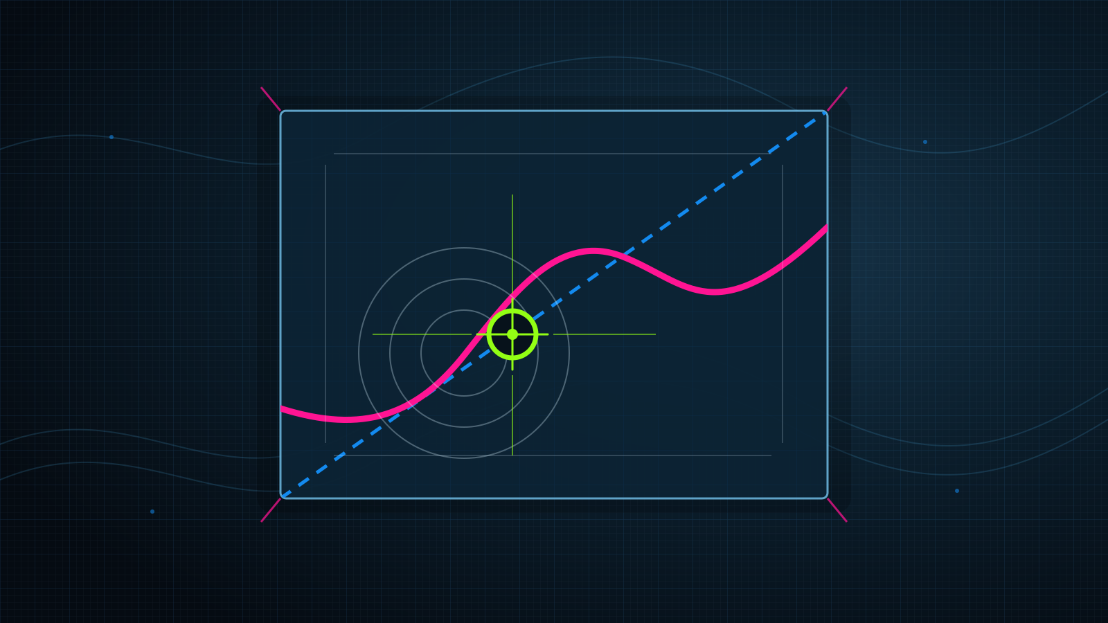
The graph of a function plots each input $x$ horizontally and its output $f(x)$ vertically. The diagonal line $y=x$ contains exactly the points whose two coordinates agree. A function therefore has a fixed point wherever its graph meets that diagonal.

Choose among three continuous functions in the diagram. The ring-and-cross marker is a shape as well as a color, so it remains identifiable without relying on the green accent.

Continuous-function explorer

Find where the output returns the input

Linear pullMirrorLogistic arch

Functionf(x) = 0.2 + 0.5x

Endpoint differenceg(0) = 0.2; g(1) = −0.3

Fixed pointx = 0.4

The logistic arch has two fixed points. The theorem promises at least one; it does not promise exactly one.

The interval theorem, stated precisely

Let $[a,b]$ be a closed interval of real numbers, including both endpoints $a$ and $b$. Suppose

$$f:[a,b]\longrightarrow[a,b]$$

is continuous. The arrow means that every input in $[a,b]$ produces an output in the same interval. Then there is at least one number $c\in[a,b]$ such that

$$f(c)=c.$$

To prove the claim, introduce a new function that measures the vertical gap between the graph of $f$ and the diagonal:

$$g(x)=f(x)-x.$$

Because $f$ and the function $x\mapsto x$ are continuous, $g$ is continuous. At the left endpoint, $f(a)$ cannot fall below $a$, because every output belongs to $[a,b]$. Therefore

$$g(a)=f(a)-a\ge 0.$$

At the right endpoint, $f(b)$ cannot rise above $b$. Therefore

$$g(b)=f(b)-b\le 0.$$

If either endpoint value equals zero, that endpoint is already fixed. Otherwise $g(a)>0$ and $g(b)<0$. The intermediate value theorem says that a continuous function taking values on opposite sides of zero must equal zero somewhere between them. Thus there is a $c\in(a,b)$ with

$$g(c)=0.$$

Substitute the definition of $g$:

$$f(c)-c=0,$$

so $f(c)=c$. That is the entire proof.

Worked example: a map pulled toward one side

Consider the function

$$f(x)=\frac15+\frac{x}{2}$$

on the interval $[0,1]$. First verify that the function sends the interval back into itself. Its smallest output occurs at $x=0$:

$$f(0)=\frac15.$$

Its largest output occurs at $x=1$:

$$f(1)=\frac15+\frac12=\frac{7}{10}.$$

Every output therefore lies between $1/5$ and $7/10$, which is inside $[0,1]$.

Now form the gap function:

$$g(x)=f(x)-x=\frac15+\frac{x}{2}-x=\frac15-\frac{x}{2}.$$

The endpoint signs point in opposite directions:

$$g(0)=\frac15>0, \qquad g(1)=\frac15-\frac12=-\frac{3}{10}<0.$$

The theorem guarantees a zero. For this linear example, solve for it directly:

$$\begin{aligned} g(x)&=0\\ \frac15-\frac{x}{2}&=0\\ \frac{x}{2}&=\frac15\\ x&=\frac25. \end{aligned}$$

Checking the result gives

$$f\!\left(\frac25\right) =\frac15+\frac12\cdot\frac25 =\frac15+\frac15 =\frac25.$$

The input $2/5$ returns unchanged.

Why each condition earns its place

The theorem can fail when one of its conditions disappears.

If the interval is open, the function

$$f(x)=\frac{x+1}{2}$$

sends every $x\in(0,1)$ back into $(0,1)$. Solving $f(x)=x$ gives $x=1$, but $1$ is missing from the open interval. The excluded endpoint takes the fixed point with it.

If continuity is removed, define $f:[0,1]\to[0,1]$ by

$$f(x)= \begin{cases} 1, & 0\le x<\tfrac12,\\ 0, & \tfrac12\le x\le1. \end{cases}$$

No input is fixed. The jump at $1/2$ lets the graph leap across the diagonal without touching it.

If outputs may leave the interval, $f(x)=x+1$ is continuous on $[0,1]$ but has no fixed point there. The requirement $f:[a,b]\to[a,b]$ is what forces the endpoint inequalities used in the proof.

Try the gap function

Problem 1

Let

$$f(x)=\frac{x+1}{3}$$

on $[0,1]$. Verify that $f$ maps the interval into itself, then find its fixed point.

Reveal the solution

At the endpoints,

$$f(0)=\frac13, \qquad f(1)=\frac23.$$

Because $f$ is increasing and linear, every output lies in $[1/3,2/3]$, which is contained in $[0,1]$.

Now solve $f(x)=x$:

$$\begin{aligned} \frac{x+1}{3}&=x\\ x+1&=3x\\ 1&=2x\\ x&=\frac12. \end{aligned}$$

Indeed, $f(1/2)=(1/2+1)/3=1/2$.

Problem 2

Why does the interval proof not apply to $f(x)=(x+1)/2$ on $(0,1)$, even though $f$ is continuous and every output stays in $(0,1)$?

Reveal the solution

The domain $(0,1)$ omits both endpoints, so the proof cannot compare $g(0)$ with $g(1)$. Direct calculation shows why that matters:

$$\frac{x+1}{2}=x \quad\Longrightarrow\quad x=1.$$

The only possible fixed point is the excluded endpoint $1$. The closed-interval condition prevents a fixed point from escaping this way.

From an interval to a room

The interval result is the one-dimensional case of Brouwer’s fixed-point theorem. In one standard form, the full theorem says:

Let $K$ be a nonempty, compact, convex subset of $\mathbb R^n$. Every continuous function $F:K\to K$ has a point $p\in K$ with $F(p)=p$.

Here, $\mathbb R^n$ is ordinary $n$-dimensional coordinate space. In this finite-dimensional setting, compact means closed and bounded. Convex means that the straight segment between any two points of $K$ remains inside $K$.

A square room is compact and convex. The position of the paper assigns every location printed on the map to a physical location inside the room. That assignment is a continuous function from the represented square back into itself. Brouwer’s theorem supplies a point whose printed coordinates and physical coordinates coincide.

The interval proof does not prove the theorem in every dimension. In higher dimensions, there is no single left endpoint and right endpoint whose signs trap a zero. The map puzzle is an application of the full theorem, while the proof above is an honest view through its one-dimensional window.

How the theorem entered mathematics

Luitzen Egbertus Jan Brouwer worked on topology—the study of properties preserved by continuous deformation—during a period when the subject’s basic language was still being built. After a 1909 visit to Paris, discussions with Henri Poincaré, Jacques Hadamard, and Émile Borel helped shape Brouwer’s work on dimension and continuous mappings. Brouwer also connected those questions to David Hilbert’s fifth problem, which asked when certain continuous transformation groups must have a differentiable structure. The University of St Andrews biography of Brouwer places these exchanges within Brouwer’s intense topological work from 1909 to 1913.

Brouwer’s 1911 paper Über Abbildung von Mannigfaltigkeiten developed the fixed-point result in the new language of manifolds and mappings. The theorem bears Brouwer’s name, but its setting grew from a network of problems and researchers working across Berlin, Göttingen, Amsterdam, and Paris—not from an isolated puzzle about maps.

Brouwer later became equally famous for intuitionism, a philosophy that rejected unrestricted use of the law of excluded middle in proofs about infinite objects. The fixed-point theorem belongs to his earlier topological program. That distinction matters because the theorem is often presented as a timeless picture, while its proof emerged amid fierce debates over what counted as a legitimate mathematical argument.

What fixed points can—and cannot—do

Fixed-point theorems are especially useful for proving that a stable state exists even when writing down that state is difficult. In 1941, Shizuo Kakutani published a generalization of Brouwer’s theorem for correspondences that may assign a set of possible outputs to one input. John Nash’s 1950 paper “Equilibrium Points in N-Person Games” used Kakutani’s theorem to prove that every finite game has at least one mixed-strategy equilibrium. At such an equilibrium, each player’s strategy is a best response to the others, so the collection of strategies returns itself under the best-response correspondence.

That application illustrates both the strength and the limit of existence theorems. A fixed-point theorem can guarantee that an equilibrium is somewhere in the allowed region. The theorem alone does not identify the equilibrium, prove that it is unique, or supply an efficient algorithm for finding it.

Numerical methods often turn equations into fixed-point searches by rewriting an equation as $x=f(x)$ and repeatedly evaluating $f$. Convergence then needs additional hypotheses, such as a contraction condition. Continuity and a closed interval guarantee existence; they do not guarantee that iteration will settle down.

One idea to remember

When a continuous function sends a closed interval back into itself, subtract the input from the output. The difference begins nonnegative and ends nonpositive, so somewhere the function must return its input unchanged.

To continue, compare the intermediate value step with how mathematics makes “close” exact, or explore contraction mappings, which add conditions strong enough to guarantee a unique fixed point and a convergent search.

Sources

• L. E. J. Brouwer, Über Abbildung von Mannigfaltigkeiten, Mathematische Annalen, volume 71, 1911, pages 97–115.
• J. J. O’Connor and E. F. Robertson, “Luitzen Egbertus Jan Brouwer”, MacTutor History of Mathematics, University of St Andrews, updated October 2003.
• Sara Ambriz, Brouwer’s Fixed Point Theorem, Directed Reading Program paper, University of California, Berkeley, Spring 2025.
• Shizuo Kakutani, “A Generalization of Brouwer’s Fixed Point Theorem”, Duke Mathematical Journal, volume 8, number 3, 1941, pages 457–459.
• John F. Nash Jr., “Equilibrium Points in N-Person Games”, Proceedings of the National Academy of Sciences, volume 36, number 1, 1950, pages 48–49.