Why Can a Particle Cross a Wall It Cannot Climb?

An electron carries $1$ electron volt of energy toward a wall that is $2$ electron volts high. Classical mechanics gives a firm verdict: the electron cannot cross. A rolling ball does not pass over a hill taller than its available energy.

Make the wall only half a nanometre thick, however, and a detector on the far side will sometimes register the electron. For the idealized barrier in this lesson, the crossing probability is about $2.35\%$.

The electron did not borrow energy to jump over the wall. Quantum mechanics asks a different question. It represents the electron with a wavefunction, and that wavefunction does not end abruptly at the barrier. The wavefunction decays inside the forbidden region. If the barrier ends before the decay has erased the wave, a transmitted wave remains on the other side. That is quantum tunneling.

The wall changes oscillation into decay

Consider motion along one horizontal coordinate $x$. Place a rectangular potential-energy barrier between $x=0$ and $x=L$:

$$U(x)= \begin{cases} 0, & x<0,\\ U_0, & 0\leq x\leq L,\\ 0, & x>L. \end{cases}$$

Here $U(x)$ is the potential energy at position $x$, $U_0$ is the barrier height, and $L$ is the barrier width. Let the particle have mass $m$ and total energy $E$, with $0<E<U_0$.

The one-dimensional, time-independent Schrödinger equation is

$$-\frac{\hbar^2}{2m}\frac{d^2\psi}{dx^2}+U(x)\psi(x)=E\psi(x).$$

The function $\psi(x)$ is the particle’s wavefunction. Its squared magnitude, $|\psi(x)|^2$, determines probability density. The constant $\hbar$ is the reduced Planck constant, and $d^2\psi/dx^2$ measures the wavefunction’s curvature.

Outside the barrier, $U(x)=0$, so $E-U(x)$ is positive. The equation permits oscillating waves, like sines and cosines. Inside the barrier, substitute $U(x)=U_0$ and rearrange:

$$\begin{aligned} -\frac{\hbar^2}{2m}\frac{d^2\psi}{dx^2}+U_0\psi&=E\psi,\\ -\frac{\hbar^2}{2m}\frac{d^2\psi}{dx^2}&=-(U_0-E)\psi,\\ \frac{d^2\psi}{dx^2}&=\frac{2m(U_0-E)}{\hbar^2}\psi. \end{aligned}$$

Define the positive decay constant

$$\kappa=\frac{\sqrt{2m(U_0-E)}}{\hbar}.$$

The equation inside the barrier becomes $\psi''=\kappa^2\psi$, whose general solution is

$$\psi(x)=Ae^{\kappa x}+Be^{-\kappa x}.$$

The constants $A$ and $B$ are fixed by requiring the wavefunction and its first derivative to join continuously at both barrier edges. The full solution contains an incoming wave, a reflected wave, and a transmitted wave. The term $e^{-\kappa x}$ supplies the central intuition: wave amplitude can penetrate a classically forbidden region, but it falls exponentially with distance.

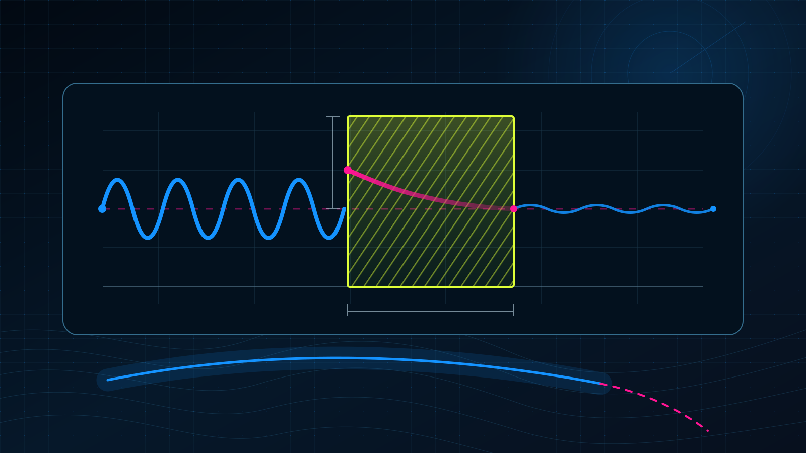
The interactive diagram below uses the electron and barrier from the opening question. The dashed horizontal line gives the electron’s energy; the top of the hatched rectangle gives the higher barrier energy.

Barrier-width sounding line

Thicken the wall and watch transmission collapse

Barrier width, L

0.50 nm

Exact transmission probability: 2.35% (about 1 in 42).

The diagram is a probability-wave picture, not a film of a little object fading and then re-forming. A single detection occurs at one place. Repeating the preparation many times reveals the reflected and transmitted probabilities.

The transmission formula

For a rectangular barrier with $E<U_0$, solving the boundary-matching equations gives the transmission probability

$$\boxed{ T=\left[1+\frac{U_0^2\sinh^2(\kappa L)}{4E(U_0-E)}\right]^{-1} }.$$

The symbol $T$ denotes the fraction of identically prepared particles expected to pass the barrier. The hyperbolic sine is $\sinh z=(e^z-e^{-z})/2$. This exact result is equivalent to the square-barrier formula derived in the Physics LibreTexts treatment of quantum tunneling.

When $\kappa L$ is appreciably larger than $1$, the growing exponential dominates $\sinh(\kappa L)$. The formula then has the useful approximation

$$\boxed{ T\approx16\frac{E}{U_0}\left(1-\frac{E}{U_0}\right)e^{-2\kappa L} }.$$

Barrier width $L$ sits in an exponent. Adding a fixed thickness therefore multiplies the probability by a fixed factor; the probability does not merely lose a fixed number of percentage points.

Worked example: a half-nanometre barrier

Take an electron with

$$E=1.00\ \text{eV},\qquad U_0=2.00\ \text{eV},\qquad L=0.500\ \text{nm}.$$

One electron volt, abbreviated eV, is the energy gained by one elementary charge across a potential difference of one volt. One nanometre, abbreviated nm, is $10^{-9}$ metres.

Step 1: calculate the energy gap.

$$U_0-E=2.00\ \text{eV}-1.00\ \text{eV}=1.00\ \text{eV}.$$

Step 2: calculate the decay constant. Using the National Institute of Standards and Technology values for the electron mass, the elementary charge, and $\hbar$,

$$\begin{aligned} \kappa &=\frac{\sqrt{2m_e(U_0-E)}}{\hbar}\\ &=5.123\times10^9\ \text{m}^{-1}\\ &=5.123\ \text{nm}^{-1}. \end{aligned}$$

The symbol $m_e$ denotes the electron mass. The last line says that each nanometre adds about $5.123$ to the dimensionless decay exponent.

Step 3: form the barrier exponent.

$$\kappa L=(5.123\ \text{nm}^{-1})(0.500\ \text{nm})=2.562.$$

Step 4: simplify the exact formula. Because $E=U_0/2$,

$$\frac{U_0^2}{4E(U_0-E)} =\frac{U_0^2}{4(U_0/2)(U_0/2)}=1.$$

Therefore

$$\begin{aligned} T &=\frac{1}{1+\sinh^2(2.562)}\\ &=\frac{1}{\cosh^2(2.562)}\\ &\approx0.02355. \end{aligned}$$

The identity $1+\sinh^2 z=\cosh^2 z$ produces the second line. Converting the decimal to a percentage gives

$$T\approx2.355\%.$$

That is roughly one transmission in every $42$ trials. The exponential approximation gives

$$T\approx4e^{-2(2.562)}\approx0.02383,$$

or $2.383\%$. The approximation differs from the exact answer by about $1.2\%$ of the exact value, which provides an independent numerical check.

From radioactive nuclei to atomic maps

Quantum tunneling became useful almost as soon as wave mechanics existed. In 1928, George Gamow and, independently, Ronald Gurney and Edward Condon applied barrier penetration to alpha decay. An alpha particle inside a nucleus lacks enough classical energy to cross the surrounding electrical barrier, but its wavefunction extends through that barrier. The small escape probability per attempt becomes a radioactive decay rate.

Gurney and Condon’s 1929 Physical Review paper emphasized that the calculation explained the Geiger–Nuttall relation across decay rates spanning roughly $10^{22}$. Gamow’s 1928 paper developed the same quantum-mechanical route independently. The episode is not a lone-genius story: two groups used the new wave mechanics to attack the same unresolved nuclear pattern.

Tunneling later became a measuring tool. In 1981, Gerd Binnig and Heinrich Rohrer developed the scanning tunneling microscope at the International Business Machines laboratory in Zürich. A sharp conducting tip is brought extremely close to a conducting surface. Electrons tunnel across the vacuum gap, and the current changes steeply when the gap changes. Holding the current fixed while moving the tip lets the instrument trace surface structure with atomic-scale sensitivity. Binnig and Rohrer shared half of the 1986 Nobel Prize in Physics for the microscope’s design.

The same exponential sensitivity that makes a barrier difficult to cross makes the microscope precise. A tiny change in distance produces a large relative change in current.

Try the exponent

Problem 1

Keep the electron energy and barrier height from the worked example, so $\kappa=5.123\ \text{nm}^{-1}$. Increase the barrier width from $0.500$ nm to $0.700$ nm. According to the exponential approximation, by what factor does the transmission probability change?

Reveal the solution

The added width is

$$\Delta L=0.700\ \text{nm}-0.500\ \text{nm}=0.200\ \text{nm}.$$

The prefactor in the approximation does not change, so the ratio is

$$\frac{T_{0.700}}{T_{0.500}} =e^{-2\kappa\Delta L} =e^{-2(5.123)(0.200)} =e^{-2.049} \approx0.1288.$$

The thicker barrier transmits about $12.9\%$ as often. Equivalently, transmission becomes about $1/0.1288\approx7.76$ times less likely. The exact formula gives $0.3065\%$ at $0.700$ nm and $2.3547\%$ at $0.500$ nm, a ratio of $0.1302$, close to the approximation.

Problem 2

For the same electron and the same energy ratio $E/U_0=1/2$, double the width from $0.500$ nm to $1.000$ nm. Use the exact formula $T=1/\cosh^2(\kappa L)$ with $\kappa=5.123\ \text{nm}^{-1}$. What percentage of particles transmit?

Reveal the solution

First compute the new exponent:

$$\kappa L=(5.123\ \text{nm}^{-1})(1.000\ \text{nm})=5.123.$$

Then

$$T=\frac{1}{\cosh^2(5.123)}\approx0.00014194.$$

Multiplying by $100$ converts the probability to a percentage:

$$T\approx0.01419\%.$$

Doubling the width does not halve the probability. It reduces the exact transmission from about $2.35\%$ to about $0.0142\%$, a factor of roughly $166$.

The idea to keep

A classically forbidden barrier turns an oscillating quantum wave into an exponential one. If the barrier is finite, the decaying wave can reach the far edge, and the surviving amplitude produces a nonzero transmission probability. Because the width appears in $e^{-2\kappa L}$, a small distance can control an enormous change in outcome.

To continue, compare this spatial exponential with the time-domain decay in Why Does Time Symmetry Keep Energy Constant? and the shrinking powers in How Can Infinitely Many Halves Stop at One?. A next quantum step is to derive the boundary-matching equations that produce the exact $T$ formula.

Sources

• Physics LibreTexts, “Quantum Tunneling of Particles through Potential Barriers”, square-barrier derivation and scanning tunneling microscope application.
• R. W. Gurney and E. U. Condon, “Quantum Mechanics and Radioactive Disintegration”, Physical Review 33, 127–140 (1929).
• George Gamow, “Zur Quantentheorie des Atomkernes”, Zeitschrift für Physik 51, 204–212 (1928).
• The Nobel Prize, “The Nobel Prize in Physics 1986”, prize motivation and scanning tunneling microscope history.
• National Institute of Standards and Technology, Fundamental Physical Constants, numerical constants used in the worked example.