How Can a Matrix Stretch a Direction Without Turning It?

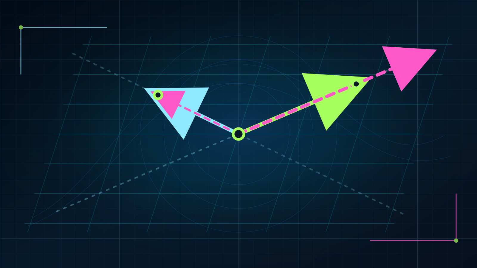
Draw an arrow from the origin on a coordinate grid. Now transform the whole grid with a matrix. Most arrows swing to a new direction. A few exceptional arrows stay on their original lines. The matrix may lengthen one of those arrows, shorten it, reverse it, or collapse it to zero, but the arrow does not leave its line.

Those exceptional directions are eigenvector directions. They reveal a transformation’s simplest behavior. Once a complicated motion has been decomposed along them, repeated transformations, coupled vibrations, and some ranking algorithms become much easier to understand.

The interactive diagram uses the matrix

$$A= \begin{pmatrix} 2&1\\ 1&2 \end{pmatrix}.$$

Move the input vector through a half-turn. The solid cyan arrow is the input vector $\mathbf v$; the dashed magenta arrow is the output $A\mathbf v$. The two faint diagonal rails mark the directions $(1,1)$ and $(1,-1)$.

Eigenvector field test

Rotate one vector through the transformation

Input angle:

45°

45° eigenvector135° eigenvector20° ordinary vector

Input v

(0.85, 0.85)

Output Av

(2.55, 2.55)

Length factor

3.00×

At 45°, the input lies on the eigenvector direction (1,1). The output is three times as long and points the same way.

input vectortransformed vectoreigenvector direction

The precise definition

A vector in the plane is an ordered pair $\mathbf v=(x,y)$. A $2\times2$ matrix acts on that vector by multiplication. For today’s matrix,

$$A\mathbf v = \begin{pmatrix} 2&1\\ 1&2 \end{pmatrix} \begin{pmatrix} x\\ y \end{pmatrix} = \begin{pmatrix} 2x+y\\ x+2y \end{pmatrix}.$$

A nonzero vector $\mathbf v$ is an eigenvector of $A$ when there is a number $\lambda$ such that

$$A\mathbf v=\lambda\mathbf v.$$

The number $\lambda$ is the eigenvalue belonging to $\mathbf v$. Multiplication by $\lambda$ changes length but keeps the vector on the same line through the origin. A positive eigenvalue preserves the arrow’s orientation, a negative eigenvalue reverses it, and a zero eigenvalue collapses the arrow to the origin.

The zero vector is excluded because every matrix sends $\mathbf 0$ to $\mathbf 0$. Calling it an eigenvector would attach every possible eigenvalue to the same uninformative vector.

First see the two locked directions

Try $\mathbf v_1=(1,1)$. Matrix multiplication gives

$$A\mathbf v_1 = \begin{pmatrix} 2(1)+1(1)\\ 1(1)+2(1) \end{pmatrix} = \begin{pmatrix} 3\\ 3 \end{pmatrix} = 3 \begin{pmatrix} 1\\ 1 \end{pmatrix}.$$

The output is three times the input, so $\mathbf v_1$ is an eigenvector with eigenvalue $\lambda_1=3$.

Now try $\mathbf v_2=(1,-1)$:

$$A\mathbf v_2 = \begin{pmatrix} 2(1)+1(-1)\\ 1(1)+2(-1) \end{pmatrix} = \begin{pmatrix} 1\\ -1 \end{pmatrix} = 1 \begin{pmatrix} 1\\ -1 \end{pmatrix}.$$

This direction is unchanged in both direction and length. Its eigenvalue is $\lambda_2=1$.

An ordinary vector behaves differently. For $\mathbf w=(1,0)$,

$$A\mathbf w= \begin{pmatrix} 2\\ 1 \end{pmatrix}.$$

The vectors $(1,0)$ and $(2,1)$ are not scalar multiples, so the horizontal direction turns.

Worked example: find the special directions instead of guessing

Guessing worked because the matrix was chosen to make the geometry visible. A systematic calculation starts from

$$A\mathbf v=\lambda\mathbf v.$$

Move the right side to the left:

$$(A-\lambda I)\mathbf v=\mathbf 0,$$

where $I$ is the identity matrix

$$I= \begin{pmatrix} 1&0\\ 0&1 \end{pmatrix}.$$

We need a nonzero solution $\mathbf v$. A homogeneous system has a nonzero solution only when its coefficient matrix is singular. The determinant lesson explains the geometry behind singularity. Here the condition is

$$\det(A-\lambda I)=0.$$

Calculate the determinant step by step:

$$\begin{aligned} \det(A-\lambda I) &= \det \begin{pmatrix} 2-\lambda&1\\ 1&2-\lambda \end{pmatrix}\\ &=(2-\lambda)(2-\lambda)-(1)(1)\\ &=(2-\lambda)^2-1\\ &=\lambda^2-4\lambda+3\\ &=(\lambda-1)(\lambda-3). \end{aligned}$$

Therefore

$$(\lambda-1)(\lambda-3)=0,$$

so the possible eigenvalues are

$$\lambda=1 \qquad\text{or}\qquad \lambda=3.$$

For $\lambda=3$,

$$A-3I= \begin{pmatrix} -1&1\\ 1&-1 \end{pmatrix}.$$

Writing $\mathbf v=(x,y)$, the first row gives

$$-x+y=0 \quad\Longrightarrow\quad y=x.$$

Every nonzero vector on the line $y=x$ is an eigenvector for $\lambda=3$. The choice $(1,1)$ is one convenient representative.

For $\lambda=1$,

$$A-I= \begin{pmatrix} 1&1\\ 1&1 \end{pmatrix}.$$

The first row gives

$$x+y=0 \quad\Longrightarrow\quad y=-x.$$

Every nonzero vector on the line $y=-x$ is an eigenvector for $\lambda=1$. The choice $(1,-1)$ is convenient.

The determinant calculation found exactly the two diagonal rails shown in the diagram.

Why repeated multiplication favors one direction

Eigenvectors make repeated matrix multiplication almost mechanical. Because

$$A\mathbf v_1=3\mathbf v_1,$$

applying $A$ again gives

$$A^2\mathbf v_1 =A(3\mathbf v_1) =3A\mathbf v_1 =3^2\mathbf v_1.$$

After $k$ applications,

$$A^k\mathbf v_1=3^k\mathbf v_1.$$

The other eigenvector satisfies

$$A^k\mathbf v_2=1^k\mathbf v_2=\mathbf v_2.$$

Any vector in the plane can be written as a combination of these two directions. For example,

$$(1,0) = \frac12(1,1)+\frac12(1,-1).$$

After $k$ applications,

$$A^k(1,0) = \frac{3^k}{2}(1,1)+\frac12(1,-1).$$

The component along $(1,1)$ grows like $3^k$, while the component along $(1,-1)$ stays fixed. Unless the original vector lies exactly on the second eigenvector line, repeated multiplication points increasingly close to $(1,1)$. The dominant eigenvalue controls the long-run direction.

Not every real matrix has a real eigenvector. A $90^\circ$ rotation turns every nonzero real vector, so no real line remains fixed. Complex numbers restore eigenvectors for that rotation, but today’s lesson stays in the real plane.

The idea came from motion before matrices

The modern notation can make eigenvectors look like an invention of matrix algebra. The motivating problems came earlier.

The MacTutor history of matrices and determinants traces an early eigenvalue problem to Jean le Rond d’Alembert’s eighteenth-century study of a vibrating string carrying attached masses. Joseph-Louis Lagrange extended the small-oscillation method: a coupled mechanical system could be decomposed into independent normal modes, with special roots determining the motions.

Augustin-Louis Cauchy’s nineteenth-century work on characteristic equations, principal axes, elasticity, and quadratic forms helped move the idea toward a general algebraic method. James Joseph Sylvester introduced the word matrix in 1850, and Arthur Cayley developed matrix algebra in the 1850s. The underlying special directions had therefore been useful before the compact object $A$ acquired its modern role.

The word eigen arrived later. It is German for “own” or “characteristic.” MacTutor’s history of the terminology records David Hilbert’s use of Eigenwert and Eigenfunktion in 1904 while studying integral equations. English texts used several alternatives—including characteristic root, latent root, and proper value—before eigenvalue and eigenvector became standard.

No lone mathematician invented the complete subject at one moment. Problems in vibrating systems, rigid-body rotation, geometry, elasticity, differential equations, and operator theory gradually exposed the same structure.

Where the locked directions do real work

Structural vibration

A bridge, wing, or spacecraft does not vibrate in an arbitrary blur. Linearized models decompose motion into normal modes. Each mode shape is represented by an eigenvector; its eigenvalue determines a natural frequency through the particular mass-and-stiffness equation being solved. A NASA technical note on vibration analysis describes eigenvalue analysis as the route to structural vibration modes.

Engineers use those modes to avoid resonance, place sensors, and understand which shapes a structure prefers when disturbed. Real structures also involve damping, nonlinear effects, joints, and uncertain material properties. The eigenvector model is a disciplined starting point, not a claim that steel and composites behave like perfect matrices.

Principal component analysis

A dataset with many correlated measurements can be difficult to picture. Principal component analysis builds a covariance matrix and finds its eigenvectors. The eigenvector with the largest eigenvalue points along the direction of greatest variance; later eigenvectors capture the greatest remaining variance while staying perpendicular to earlier directions. The University of Illinois numerical-methods text derives that relationship.

The method can compress images, visualize high-dimensional measurements, and reduce the number of variables used by a model. Principal component analysis preserves directions with large variance, not necessarily directions with the most meaning or predictive value.

Ranking a network

PageRank models movement through a network of linked pages. With damping and teleportation included, the long-run distribution is a principal eigenvector of the transition matrix with eigenvalue $1$. Stanford’s information-retrieval text explains how the entries of that eigenvector become PageRank scores.

The connection is the repeated-multiplication effect from the previous section. Applying the transition matrix again and again suppresses transient components and approaches the stable eigenvector. Modern search engines use many signals beyond the original PageRank formulation, but the algorithm remains a clean example of an eigenvector encoding equilibrium.

Try the calculation

Problem 1

Let

$$B= \begin{pmatrix} 4&0\\ 0&2 \end{pmatrix}.$$

Find its eigenvalues and describe the corresponding eigenvector directions.

Reveal the solution

Start with the characteristic equation:

$$\begin{aligned} \det(B-\lambda I) &= \det \begin{pmatrix} 4-\lambda&0\\ 0&2-\lambda \end{pmatrix}\\ &=(4-\lambda)(2-\lambda). \end{aligned}$$

Therefore the eigenvalues are $\lambda=4$ and $\lambda=2$.

For $\lambda=4$,

$$(B-4I)\mathbf v = \begin{pmatrix} 0&0\\ 0&-2 \end{pmatrix} \begin{pmatrix} x\\ y \end{pmatrix} = \mathbf 0,$$

so $y=0$ and $x$ may be any nonzero number. The eigenvector direction is the horizontal axis, represented by $(1,0)$.

For $\lambda=2$,

$$(B-2I)\mathbf v = \begin{pmatrix} 2&0\\ 0&0 \end{pmatrix} \begin{pmatrix} x\\ y \end{pmatrix} = \mathbf 0,$$

so $x=0$ and $y$ may be any nonzero number. The eigenvector direction is the vertical axis, represented by $(0,1)$.

Problem 2

For the lesson’s matrix $A$, calculate $A^3(1,0)$ in two ways: by three direct multiplications and by the eigenvector decomposition

$$(1,0)=\frac12(1,1)+\frac12(1,-1).$$

Reveal the solution

Direct multiplication gives

$$\begin{aligned} A(1,0)&=(2,1),\\ A^2(1,0)&=A(2,1)=(5,4),\\ A^3(1,0)&=A(5,4)=(14,13). \end{aligned}$$

For the eigenvector method, $(1,1)$ has eigenvalue $3$ and $(1,-1)$ has eigenvalue $1$. Therefore

$$\begin{aligned} A^3(1,0) &=\frac12\,3^3(1,1)+\frac12\,1^3(1,-1)\\ &=\frac{27}{2}(1,1)+\frac12(1,-1)\\ &=\left(\frac{28}{2},\frac{26}{2}\right)\\ &=(14,13). \end{aligned}$$

Both methods agree. The decomposition turns repeated matrix multiplication into repeated multiplication by two ordinary numbers.

The idea to keep

An eigenvector is a nonzero direction that a linear transformation does not turn; its eigenvalue records the stretch, shrink, reversal, or collapse along that direction. These directions matter because they separate coupled behavior into independent pieces.

Continue with Why Does $ad-bc$ Measure Area? for the determinant behind the characteristic equation, or Can a Random Process Forget Where It Started? for a probability process whose long-run state is an eigenvector.

Sources

• Massachusetts Institute of Technology OpenCourseWare, “Eigenvalues and Eigenvectors”, definition and calculation of eigenvectors and eigenvalues.
• J. J. O’Connor and E. F. Robertson, “Matrices and Determinants”, MacTutor History of Mathematics, historical development from mechanical systems to matrix algebra.
• Jeff Miller, “Earliest Known Uses of Some of the Words of Mathematics: E”, MacTutor History of Mathematics, the 1904 eigenvalue terminology.
• National Aeronautics and Space Administration, technical note on vibration modes and eigenvalue analysis.
• University of Illinois Urbana-Champaign, CS 357, “Principal Component Analysis”.
• Stanford University, Introduction to Information Retrieval, “The PageRank Computation”.